Hyperspectral Image Preprocessing with Python
This is the preliminary prerequisites you need if you want to build a hyperspectral preprocessing system using Python.
- Knowledge of hyperspectral imaging
- Anaconda
- SpectralPy
- RAW and HDR file from hyperspectral camera (in this post using Specim FX-10)
As usual we import the required modules, we use spectral library for opening files, numpy for numerical processing and matplotlib for visualization.
from spectral import imshow, view_cube
import spectral.io.envi as envi
import numpy as np
import matplotlib.pyplot as plt
import matplotlib
Using envi.open() function we open both RAW and HDR file, we need three type of data here: dark reference, white reference and data capture. In my experiment I use Specim FX-10 hyperspectral camera, that produce this results (dark reference and white reference).
dark_ref = envi.open('path/to/dark_reference.hdr', 'path/to/dark_reference.raw')
white_ref = envi.open('path/to/white_reference.hdr', 'path/to/white_reference.raw')
data_ref = envi.open('path/to/data_capture.hdr', 'path/to/data_capture.raw')
With numpy, we convert the loaded data to numpy array tensor, as oposed of standard Python array.
white_nparr = np.array(white_ref.load())
dark_nparr = np.array(dark_ref.load())
data_nparr = np.array(data_ref.load())
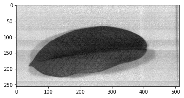
Using correction formula, the captured data is subtracted by dark reference and divided with white reference subtracted dark reference. To show our currently corrected image, use imshow from spectral library.
corrected_nparr = np.divide(
    np.subtract(data_nparr, dark_nparr),
    np.subtract(white_nparr, dark_nparr))

imshow(corrected_nparr, (100, 100, 100))
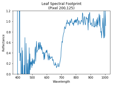
Since hyperspectral camera have a lot of bands (commonly called channels in RGB image, bands contain a list of wavelength measured in nanometer) within a single image we can create a figure where we can plot a reflectance versus the bands itself. With this file that represent each value of spectral bands we can display each pixel spectral features as figured with reflectance versus wavelength.
bands = np.genfromtxt('bands.csv', delimiter=',')
Using selected pixel by defining its coordinae we can call the pixel vector from above corrected hyperspectral tensor. Then we squeeze to acquire un-arrayed elements of vector. At last, we could plot its spectral footprint.
leaf_pixel_y = 75
leaf_pixel_x = 200

leaf_pixel = corrected_nparr[
    leaf_pixel_y:leaf_pixel_y+1,
    leaf_pixel_x:leaf_pixel_x+1,
    :]

leaf_pixel_squeezed = np.squeeze(leaf_pixel)

plt.plot(bands, leaf_pixel_squeezed)
plt.title('Leaf Spectral Footprint\n(Pixel {},{})'.format(
    leaf_pixel_x, leaf_pixel_y))
plt.xlabel('Wavelength')
plt.ylabel('Reflectance')
plt.show()
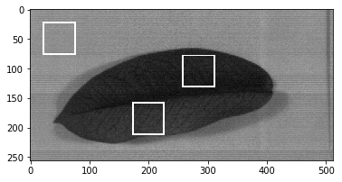
The ROIs (region of interests) coordinate is the coordinate where you want to select a certain object within an image, for example, in my case I select the leaf and board objects. The coordinate itself is top-left of a bounding box, measured in pixels. To acquire ROI that we will use for processing phase (training phase) we can extract the ROI by using bounding box method. Let’s build a function that do that.
def extract_roi(arr, x, y, w, h, intensity, line):
    roi = arr[y:y+h, x:x+w, :]

    bounding_box = arr
    bounding_box[y-line:y, x-line:x+w+line, :] = intensity # top line
    bounding_box[y:y+h, x-line:x, :] = intensity # left line
    bounding_box[y+h:y+h+line, x-line:x+w+line, :] = intensity # bottom line
    bounding_box[y:y+h, x+w:x+w+line, :] = intensity # right line

    return (roi, bounding_box)
Next, we need the coordinates that define where the bounding boxes belong.
coordinates = [
    (105, 65),
    (120, 60),
    (160, 65)
]
rois = [] # returned ROIs
length = 50 # width and height
line = 0 # bounding box line width
intensity = 2 # bounding box line intensity
image_bboxed = None

for coordinate in coordinates:
    (x, y) = coordinate
    (roi, image_bboxed) = extract_rois(
        corrected_nparr, x, y, length, length, intensity, line)
    rois.append(roi)

imshow(image_bboxed, (100, 100, 100))
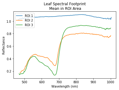
Finally, to get the averaged spectral features in each boxes we could use the np.mean() function.
for i in range(len(rois)):
    roi = rois[i]
    intensity = []
    for b in range(roi.shape[2]):
        intensity.append(np.mean(roi[:, :, b]))
    plt.plot(bands, intensity, label='ROI {}'.format(i+1))

plt.legend(loc='upper left')
plt.title('Leaf Spectral Footprint\n Mean in ROI Area')
plt.xlabel('Wavelength (nm)')
plt.ylabel('Reflectance')
plt.show()
Now we are finished with a rois variable that we can save as .npy, with this data we can continue to the processing phase.
np.save("rois.npy", rois)